seg_plot class and methods

A seg_plot is an object to plot data associated with a dna_seg object. It is a list with mandatory and optional arguments. The main arguments are func, which is a function that returns a grob or a gList, and args, which are arguments to be passed to this function.

Usage

seg_plot(
  func,
  args = NULL,
  xargs = c("x", "x0", "x1", "x2", "v"),
  yargs = c("y", "y0", "y1", "y2", "h"),
  ylim = NULL
)

as.seg_plot(seg_plot)

is.seg_plot(seg_plot)

Arguments

func

A function that returns a grob or a gList list of grobs. User-defined functions can be used, but ready-made functions from the grid package can be used as well.

args

A list, NULL by default. The arguments that will be passed to the function. It is recommended that all arguments are named.

xargs

A character vector containing the names of the arguments from args that define the x-axis. Used, among others, by the function trim.seg_plot. By default, gives the most common x-defining arguments of the grid functions (x, x0, x1, x2, v).

yargs

A character vector containing the names of the arguments from args that define the y-axis. Used when plotting the graphs to define a sensible ylim if not defined. By default, gives the most common y-defining arguments of the grid functions (y, y0, y1, y2, h).

ylim

A numeric vector of length 2, defining the range of the plot when drawn with plot_gene_map. Derived from yargs if not set.

seg_plot

In as.seg_plot, a list object to convert to seg_plot. The list must consist of named elements matching the above arguments, with func and args being mandatory. See details below.

In is.seg_plot, an object to test.

Value

seg_plot and as.seg_plot return a seg_plot object. is.seg_plot returns a logical.

Details

A seg_plot object is an object describing how to plot data associated to a dna_seg. It is a list composed of a function, arguments to pass to this function, two arguments to define which of those define x and y, and an eventual ylim to limit the plotting to a certain range.

Internally, the seg_plot function calls as.seg_plot using a list with the arguments of seg_plot as named elements. In other words, the input to as.seg_plot should be a list with at least func and args as named elements, with xargs, yargs, and ylim as optional named elements.

The function func should return a grob object, or a gList list of grobs. The predefined functions of grid can be used, such as linesGrob, pointsGrob, segmentsGrob, textGrob, or polygonGrob. Alternatively, user-defined functions can be used instead.

The arguments in args should correspond to arguments passed to func. For example, if func = pointsGrob, args could contain the elements x = 10:1, y = 1:10. It will often also contain a gp element, the result of a call to the gpar function, to control graphical aspects of the plot such as color, fill, line width and style, fonts, etc.

is.seg_plot returns TRUE if the object tested is a seg_plot object.

Author

Lionel Guy

Examples

## Using the existing pointsGrob
x <- 1:20
y <- rnorm(20)
sp <- seg_plot(func = pointsGrob, 
               args = list(x = x, y = y, gp = gpar(col = 1:20, cex = 1:3)))
is.seg_plot(sp)
#> [1] TRUE
## Function seg_plot(...) is identical to as.seg_plot(list(...))
sp2 <- as.seg_plot(list(func = pointsGrob,
                        args = list(x = x, y = y,
                                    gp = gpar(col = 1:20, cex = 1:3))))
identical(sp, sp2)
#> [1] FALSE
## For the show, plot the obtained result
grb <- do.call(sp$func, sp$args)
## Trim the seg_plot
sp_trim <- trim(sp, c(3, 10))
## Changing color and function "on the fly"
sp_trim$args$gp$col <- "blue"
sp_trim$func <- linesGrob
grb_trim <- do.call(sp_trim$func, sp_trim$args)
## Now plot
plot.new()
pushViewport(viewport(xscale = c(0, 21), yscale = c(-4, 4)))
grid.draw(grb)
grid.draw(grb_trim)


## Using home-made function
triangleGrob <- function(start, end, strand, col, ...) {
  x <- c(start, (start+end)/2, end)
  y1 <- 0.5 + 0.4*strand
  y <- c(y1, rep(0.5, length(y1)), y1)
  polygonGrob(x, y, gp = gpar(col = col), default.units = "native",
              id = rep(1:7, 3))
}
start <- seq(1, 19, by = 3) + rnorm(7) / 3
end <- start + 1 + rnorm(7)
strand <- sign(rnorm(7))
sp_tr <- seg_plot(func = triangleGrob,
                  args = list(start = start, end = end, strand = strand,
                            col = 1:length(start)),
                  xargs = c("start", "end"))
grb_tr <- do.call(sp_tr$func, sp_tr$args)
plot.new()
pushViewport(viewport(xscale = c(1, 22), yscale = c(-2, 2)))
grid.draw(grb_tr)

## Trim
sp_tr_trim <- trim(sp_tr, xlim = c(5, 15))
str(sp_tr_trim)
#> List of 5
#>  $ func :function (start, end, strand, col, ...)  
#>  $ args :List of 5
#>   ..$ start        : num [1:2] 7.89 9.88
#>   ..$ end          : num [1:2] 7.72 9.9
#>   ..$ strand       : num [1:2] 1 1
#>   ..$ col          : int [1:2] 3 4
#>   ..$ default.units: chr "native"
#>  $ xargs: chr [1:2] "start" "end"
#>  $ yargs: chr [1:5] "y" "y0" "y1" "y2" ...
#>  $ ylim : NULL
#>  - attr(*, "class")= chr [1:2] "seg_plot" "list"
## If the correct xargs are not indicated, trimming won't work
sp_tr$xargs <- c("x")
sp_tr_trim2 <- trim(sp_tr, xlim = c(5, 15))
identical(sp_tr_trim, sp_tr_trim2)
#> [1] FALSE

y1 <- convertY(grobY(grb_tr, "south"), "native")
y2 <- convertY(grobY(grb_tr, "north"), "native")
heightDetails(grb)
#> [1] 7.77856344394176inches
grb
#> points[GRID.points.54] 

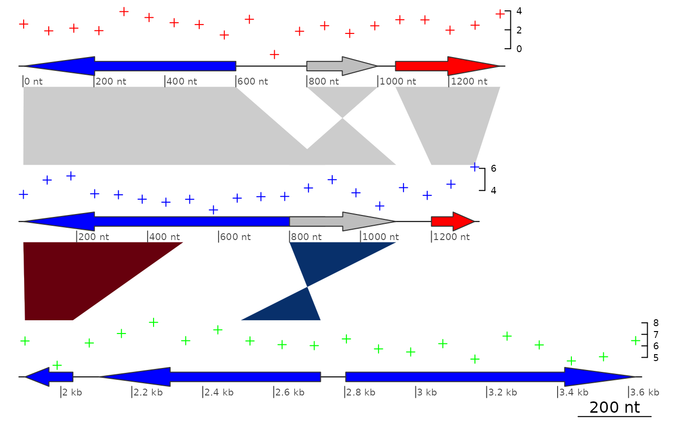
## Applying it to plot_gene_maps
data(three_genes)
dna_segs <- three_genes$dna_segs
comparisons <- three_genes$comparisons

## Build data to plot
xs <- lapply(dna_segs, range)
colors <- c("red", "blue", "green")

seg_plots <- list()
for (i in 1:length(xs)) {
  x <- seq(xs[[i]][1], xs[[i]][2], length = 20)
  seg_plots[[i]] <- seg_plot(func = pointsGrob,
                             args = list(x = x, y = rnorm(20) + 2 * i,
                             default.units = "native", pch = 3,
                             gp = gpar(col = colors[i], cex = 0.5)))
}
plot_gene_map(dna_segs, comparisons,
              seg_plots = seg_plots,
              seg_plot_height = 0.5,
              seg_plot_height_unit = "inches",
              dna_seg_scale = TRUE)


## A more complicated example
data(barto)
tree <- ade4::newick2phylog("(BB:2.5,(BG:1.8,(BH:1,BQ:0.8):1.9):3);")
## Showing several subsegments per genome
xlims2 <- list(c(1445000, 1415000, 1380000, 1412000),
               c(  10000,   45000,   50000,   83000, 90000, 120000),
               c(  15000,   36000,   90000,  120000, 74000,  98000),
               c(   5000,   82000))

## Adding fake data in 1kb windows
seg_plots <- lapply(barto$dna_segs, function(ds) {
  x <- seq(1, range(ds)[2], by = 1000)
  y <- jitter(seq(100, 300, length = length(x)), amount = 50)
  seg_plot(func = linesGrob,
           args = list(x = x, y = y, gp = gpar(col = grey(0.3), lty = 2)))
})
plot_gene_map(barto$dna_segs, barto$comparisons, tree = tree,
              seg_plots = seg_plots,
              seg_plot_height = 0.5,
              seg_plot_height_unit = "inches",
              xlims = xlims2,
              limit_to_longest_dna_seg = FALSE,
              dna_seg_scale = TRUE,
              main = "Random plots for the same segment in 4 Bartonella genomes")